The Mathematics of Expertise in the Age of AI

For the last year, I have been trying to understand something that does not quite add up.

If AI is replacing expertise, why does expertise still matter so much?

AI is making professional work accessible to people who previously lacked the skills to do it. Research shows that novices and less-experienced workers can experience larger productivity gains from AI than experts do. But a larger improvement is not necessarily a better final result. And a better individual result is not the same as a reliable production system. [1–3]

A novice might improve dramatically and still fall short of the standard a business needs. An expert might improve less, relatively speaking, and still produce higher-quality work. Even that is not guaranteed: on some tasks AI narrows the gap, and in some settings it can degrade experienced workers’ quality. The answer depends on the task, the person, the system and what we are measuring. [2, 3]

That leaves me with a question more useful than “who gets the bigger AI boost?”

What happens to expertise when we measure both the amount of work produced and the quality, reliability and commercial value of what gets shipped?

Notation20 symbols. Point at any highlighted symbol in the text to see what it means.

Symbol	Meaning	Units or range
$\mathcal{D}$	The design space: every possible design decision. Every layout, type scale, colour combination, spacing system, image treatment and motion curve.	A set. Enormous and unconstrained.
$d$	One design: a single point in $\mathcal{D}$ .	$d \in \mathcal{D}$
$c$	One specific context: the brand, audience, channel, accessibility requirement and legal context a design is for.	One context; each has its own rules.
$c_1, c_2$	Two example contexts in the figures: a fashion campaign and a safety notice.	Two contexts.
$r_i(d, c)$	Inequality rule number $i$ : a non-negotiable requirement with a threshold, such as a contrast rule, written so that it holds when $r_i(d, c) \le 0$ .	A number in the rule’s own units (a ratio, characters, pixels). Met at $0$ or below.
$h_j(d, c)$	Equality rule number $j$ : a non-negotiable requirement with one exact value, such as a required disclosure or an approved format. It holds only when $h_j(d, c) = 0$ .	A number. Met only at exactly $0$ .
$\mathcal{F}(c)$	The feasible region: every design in $\mathcal{D}$ that meets every non-negotiable rule of context $c$ .	A subset of $\mathcal{D}$ . It changes with $c$ .
$U(d, c)$	The evaluation function: how valuable design $d$ is in context $c$ .	A number. Higher is better. No fixed scale; the figures use $0$ to $1$ .
$B(d, c)$	Brand fit.	A score. Higher is better.
$L(d, c)$	Clarity, or legibility.	A score. Higher is better.
$A(d, c)$	Aesthetic quality.	A score. Higher is better.
$P(d, c)$	Expected performance: an estimate until actual results arrive.	A score. Higher is better.
$\alpha, \beta, \gamma, \delta$	The weights on $B$ , $L$ , $A$ and $P$ : the priorities of the context, not objective truths.	Weights of $0$ or more, set per context. The figures make them add up to $1$ .
$d^*$	The best permitted design: the one in $\mathcal{F}(c)$ with the highest value.	A member of $\mathcal{F}(c)$ .
$d_1, d_2, d_3, \ldots$	Individual outputs, made one at a time.	Designs.
$N$	The number of approved assets.	A count.
$H$	Total human effort: production, review, correction, approval and an allocated share of setup and maintenance.	Hours.
$\mathrm{CVR}$	Constraint Violation Rate: the share of submitted assets that fail at least one mandatory rule on the first pass.	$0$ to $1$ (0% to 100%). Lower is better.
$\mathrm{ERL}$	Expert Review Load: expert review minutes per approved asset.	Minutes per asset. Lower is better.
$\mathrm{NFA}$	Non-expert First-pass Acceptance: the share of non-expert assets accepted on the first pass.	$0$ to $1$ (0% to 100%). Higher is better.

Notation	Read it as
$\in$	“Is in”. $d \in \mathcal{F}(c)$ reads “ $d$ is in the feasible region”.
$r_i,\ h_j,\ c_1$	A small letter or number below a symbol says which one it is: $r_i$ is rule number $i$ .
$\{\, d \in \mathcal{D} \mid \ldots \,\}$	“The set of designs $d$ in $\mathcal{D}$ such that …”.
$\le 0,\ = 0$	“Zero or less” and “exactly zero”. Every rule is written so it can be checked against zero.
$\arg\max$	“The design that makes … largest.” It gives back a design, not a score.

An improvement is not an outcome

Imagine two people using the same AI system. Before AI, a novice scores 45 out of 100 on a hypothetical quality rubric; afterward, 60. An expert moves from 70 to 85. The novice improves by 33%. The expert improves by roughly 21%. If commercial approval requires 80, only the expert crosses the threshold.

These numbers are an illustration, not findings from a study. They demonstrate a distinction that relative percentage gains can conceal: uplift, final quality and acceptable output are three different measurements.

This distinction matters because commercial work has cliffs. An advertisement that is 95% compliant may still be unusable if the missing 5% is a legally required disclaimer. A beautifully composed asset can be rejected for an unlicensed image or the wrong product claim. Small errors can have consequences out of proportion to their visual size.

The studies should be read carefully. Noy and Zhang found that ChatGPT reduced completion time on professional writing tasks by 40% and increased independently rated quality by 18%, while narrowing differences between workers. Brynjolfsson, Li and Raymond observed a 15% average productivity gain across 5,172 support agents; less-experienced agents gained more, while the most experienced had slight speed gains and slight quality declines. Dell’Acqua and colleagues found that AI helped consultants on tasks inside its capability frontier and hurt performance on some tasks outside it. These findings do not demonstrate universal expert superiority. They demonstrate why we have to measure speed and quality together. [1–3]

The design space

Imagine every possible design decision: every layout, type scale, colour combination, spacing system, image treatment and motion curve. Let $\htmlData{term=design-space}{\mathcal{D}}$ represent that enormous design space.

A generative model can produce plausible candidates from statistical patterns and instructions. But plausibility is not the same as suitability. A generated landing page may look impressive and be wrong for the brand, audience, channel, accessibility requirement or legal context.

Represent that specific context by $\htmlData{term=context}{c}$ . A useful production system must account for context rather than assume a universal definition of “good”. This is the core connection between design judgment and optimisation. Work on constrained graphic layouts and computational design spaces shows how constraints and structured decision spaces can support automated exploration. [5, 6]

Define what is permitted

Some requirements are non-negotiable. A logo needs clear space. A required disclosure must appear. Text must satisfy a specified contrast rule. An export has to use an approved format. Other requirements are negotiable: a headline may be bolder, imagery may be more expressive, or a composition may trade novelty for familiarity.

The non-negotiable rules can be represented as equalities and inequalities:

Equation 1

\htmlData{term=inequality}{r_i(d, c)} \htmlData{term=zero}{\le 0} \qquad \text{and} \qquad \htmlData{term=equality}{h_j(d, c)} \htmlData{term=zero}{= 0}

Together they define the feasible region for context $\htmlData{term=context}{c}$ :

Equation 2

\htmlData{term=feasible-region}{\mathcal{F}(c)} = \{\, \htmlData{term=design}{d} \htmlData{term=is-in}{\in} \htmlData{term=design-space}{\mathcal{D}} \htmlData{term=such-that}{\mid} \htmlData{term=inequality}{r_i(d, c)} \htmlData{term=zero}{\le 0} \text{ and } \htmlData{term=equality}{h_j(d, c)} \htmlData{term=zero}{= 0} \,\}

Three number lines, one per rule. Text contrast of at least 4.5:1: everything from 4.5:1 up is allowed. Headline of at most 60 characters: everything from 0 to 60 is allowed. Aspect ratio of exactly 4:5: only that single point is allowed. — An inequality, $\htmlData{term=inequality}{r_i(d, c)} \htmlData{term=zero}{\le 0}$ , allows a whole range, up to and including its threshold. An equality, $\htmlData{term=equality}{h_j(d, c)} \htmlData{term=zero}{= 0}$ , allows one exact value: it has to be set, not approximated.

The distinction is operational, not just mathematical. Putting a rule in a prompt does not enforce it. A production system needs a way to check it, block or repair violations, document exceptions and escalate ambiguous cases. Some checks can be deterministic; others need an AI reviewer or a human, and those reviewers can make mistakes too.

The goal is not to prevent exploration. It is to prevent exploration from quietly becoming noncompliant production.

Headline length plotted against text contrast ratio. The fashion campaign’s feasible region allows contrast from 3:1 and headlines up to 40 characters. The safety notice’s region allows contrast from 7:1 and headlines up to 80 characters. A design d, at 5:1 contrast with a 14-character headline, sits inside the fashion campaign’s region and outside the safety notice’s. — Each context sets its own thresholds, so each has its own feasible region. The same design $\htmlData{term=design}{d}$ is permitted for the fashion campaign, $\htmlData{term=example-contexts}{c_1}$ , and not for the safety notice, $\htmlData{term=example-contexts}{c_2}$ . Illustrative thresholds.

Feasible does not mean excellent

A design can satisfy every brand rule and still be forgettable. Constraint satisfaction tells us whether an output is allowed; it does not tell us whether it is the best permitted option.

For that we need a context-dependent evaluation function, $\htmlData{term=evaluation}{U(d, c)}$ . It might combine brand fit, clarity, aesthetics and expected performance:

Equation 3

\htmlData{term=evaluation}{U(d, c)} = \htmlData{term=weights}{\alpha} \htmlData{term=brand}{B(d, c)} + \htmlData{term=weights}{\beta} \htmlData{term=clarity}{L(d, c)} + \htmlData{term=weights}{\gamma} \htmlData{term=aesthetics}{A(d, c)} + \htmlData{term=weights}{\delta} \htmlData{term=performance}{P(d, c)}

The weights express priorities, not objective truths. A safety notice may prioritise clarity over originality. A fashion campaign may reverse that balance. Predicted campaign performance is an estimate until actual results arrive, and different qualified reviewers may disagree about aesthetic quality. The DesignPref research found substantial disagreement among professional designers, a warning against treating taste as a single universal number. [7]

Stacked bars splitting utility into its four weighted parts, for two designs in two contexts. Safety notice, with weights alpha 0.2, beta 0.45, gamma 0.15 and delta 0.2: design a, plain and highly legible, scores 0.77; design b, bold and expressive, scores 0.67. Fashion campaign, with weights alpha 0.25, beta 0.15, gamma 0.4 and delta 0.2: design a scores 0.66; design b scores 0.80. — Same two designs, same scores, different weights. Weighting legibility picks the plain design; weighting aesthetics picks the expressive one. The higher $\htmlData{term=evaluation}{U(d, c)}$ in each context is in blue. Illustrative numbers.

The design objective can now be written:

Equation 4

\htmlData{term=best-design}{d^*} = \htmlData{term=arg-max}{\arg\max}\, \htmlData{term=evaluation}{U(d, c)} \qquad \text{subject to } \htmlData{term=design}{d} \htmlData{term=is-in}{\in} \htmlData{term=feasible-region}{\mathcal{F}(c)}

In plain English: among the designs that satisfy the requirements, seek the one with the highest value for the context. This equation formalises the decision problem. It does not prove that any particular AI system will solve it, or that a particular expert has defined the right function.

The design with the highest utility overall breaks the contrast rule. $\htmlData{term=best-design}{d^*}$ is the best design that doesn’t: it sits where the highest ring still touching $\htmlData{term=feasible-region}{\mathcal{F}(c)}$ meets it, on the region’s edge. Illustrative numbers.

The two gains that matter

The first gain is individual productivity: how much faster someone completes a task, and whether their final result is better. We should measure both dimensions, rather than hide them inside one ambiguous score.

A novice often asks the model to search the full design space, $\htmlData{term=design-space}{\mathcal{D}}$ . They generate an output and hope it happens to be good.

An expert brings a much clearer understanding of:

the context
the constraints
the acceptable tradeoffs
the quality bar
the likely failure modes

They reduce the search space to something closer to $\htmlData{term=feasible-region}{\mathcal{F}(c)}$ .

They are not necessarily better because they can write more elaborate prompts. They are better because they know how to define the problem.

The model generates possibilities. The expert determines which possibilities should exist in the first place.

The same model, 40 tries each. Searching all of $\htmlData{term=design-space}{\mathcal{D}}$ lands 19 designs inside $\htmlData{term=feasible-region}{\mathcal{F}(c)}$ ; starting from the expert’s constraints lands 35. Illustrative numbers.

The second gain is systems leverage: can an expert make the quality standard repeatable across many outputs, users and agents? Instead of personally producing $\htmlData{term=outputs}{d_1}$ , $\htmlData{term=outputs}{d_2}$ , $\htmlData{term=outputs}{d_3}$ and so on, an expert might define the permitted set $\htmlData{term=feasible-region}{\mathcal{F}(c)}$ , shape the evaluation criteria $\htmlData{term=evaluation}{U(d, c)}$ , and decide when automated production must stop for review.

This is not merely “better prompting”. It involves workflow design, reusable components, policy versioning, monitoring, fallback behaviour, exception routing and an understanding of the downstream consequences of mistakes. It also requires maintenance as brands, regulations and channels change.

Importantly, domain expertise and systems-design expertise are not identical. A great designer is not automatically a great automation architect. The stronger unit may be a collaboration: domain experts, product and systems engineers, compliance specialists, and the operators who work with the process every day.

Nor are autonomous systems automatically superior because an expert initiated them. Autonomy scales good decisions and bad assumptions alike. A flawed policy replicated across thousands of assets can be more damaging than a one-off mistake. The economic argument for verification becoming a bottleneck is articulated by Catalini, Hui and Wu, but their 2026 paper is a theoretical working paper, not direct evidence that any one creative platform solves the problem. [8]

Quality-adjusted productivity

To test this properly, count the outputs that actually meet a pre-agreed standard, not merely the outputs a system generates.

Equation 5

\text{Accepted throughput} = \frac{\htmlData{term=approved}{N}}{\htmlData{term=hours}{H}} = \frac{\text{Approved assets}}{\text{Human hours}}

Here $\htmlData{term=approved}{N}$ is the number of approved assets and $\htmlData{term=hours}{H}$ is the total human effort, including production, review, correction, approval and an allocated share of setup and maintenance. Report elapsed time alongside it; a system can consume little human effort yet be too slow to use commercially.

A second metric captures the economic side:

Equation 6

\text{Cost per accepted asset} = \frac{\text{Total costs}}{\htmlData{term=approved}{N}}

The numerator includes generation, review, rework and an allocated share of configuration and maintenance costs. Without that final component, automation appears cheaper than it really is.

Quality needs several lenses. First, does the asset satisfy the mandatory requirements? Second, how well does it perform against an independent, blinded quality rubric? Third, when evidence is available, how does it perform in the actual channel or business context? An approval rate cannot replace all three. A workflow that doubles generation but also doubles failures has not necessarily improved production.

Commercial risk also belongs in the model. A critical failure must not be treated as interchangeable with an ordinary spacing correction. At minimum, track severity-weighted incidents, escaped defects, false approvals and time-to-remediation. Where reliable probabilities and financial impacts exist, expected loss can be estimated as a sum of probability multiplied by consequence. When those estimates do not exist, do not manufacture precision.

Three measurements for a serious test

1. Constraint Violation Rate (CVR)

Equation 7

\htmlData{term=cvr}{\mathrm{CVR}} = \frac{\text{Assets failing} \ge 1 \text{ mandatory rule on first pass}}{\text{All submitted assets}}

Run the same independently validated rules on every experimental group. Report severe violations separately from minor ones, and audit the checker’s false positives and false negatives. This corrects an ambiguity in the original formula, which reused D for both the entire design space and the observed batch.

Two grids of 40 squares, one square per asset. Without the constraint set, 14 squares are outside the feasible region: CVR = 14/40 = 35%. With the constraint set encoded, 2 are outside: CVR = 2/40 = 5%. — CVR counts the assets outside $\htmlData{term=feasible-region}{\mathcal{F}(c)}$ (the open squares) and divides by all submitted assets. On its own, 5% means little: the paired baseline, checked by the same rules, is what gives it meaning. Illustrative numbers.

2. Expert Review Load (ERL)

Equation 8

\htmlData{term=erl}{\mathrm{ERL}} = \frac{\text{Expert review minutes}}{\text{Approved assets}}

Track revision cycles and the time required to create and maintain constraints separately. A lower review load is meaningful only if the acceptance standard remains constant.

Line chart of expert minutes per approved asset against the number of approved assets. Without the constraint set, review takes 12 minutes per asset. With it, review alone takes 4 minutes, a dashed line. Adding 10 hours of authoring, shared across the assets, gives a curve that starts high, crosses 12 minutes at 75 assets and then falls towards 4. — Count review time alone and the constrained system looks like 4 minutes per asset from day one. Share the 10 hours spent writing $\htmlData{term=feasible-region}{\mathcal{F}(c)}$ across the assets it governs, and it only beats the baseline after 75 assets. Illustrative numbers.

3. Non-expert First-pass Acceptance (NFA)

Equation 9

\htmlData{term=nfa}{\mathrm{NFA}} = \frac{\text{First-pass accepted non-expert assets}}{\text{All non-expert assets}}

Define “material revision” before evaluation. Compare the same non-expert operators with and without expert-authored controls, and evaluate all submissions against a blinded standard.

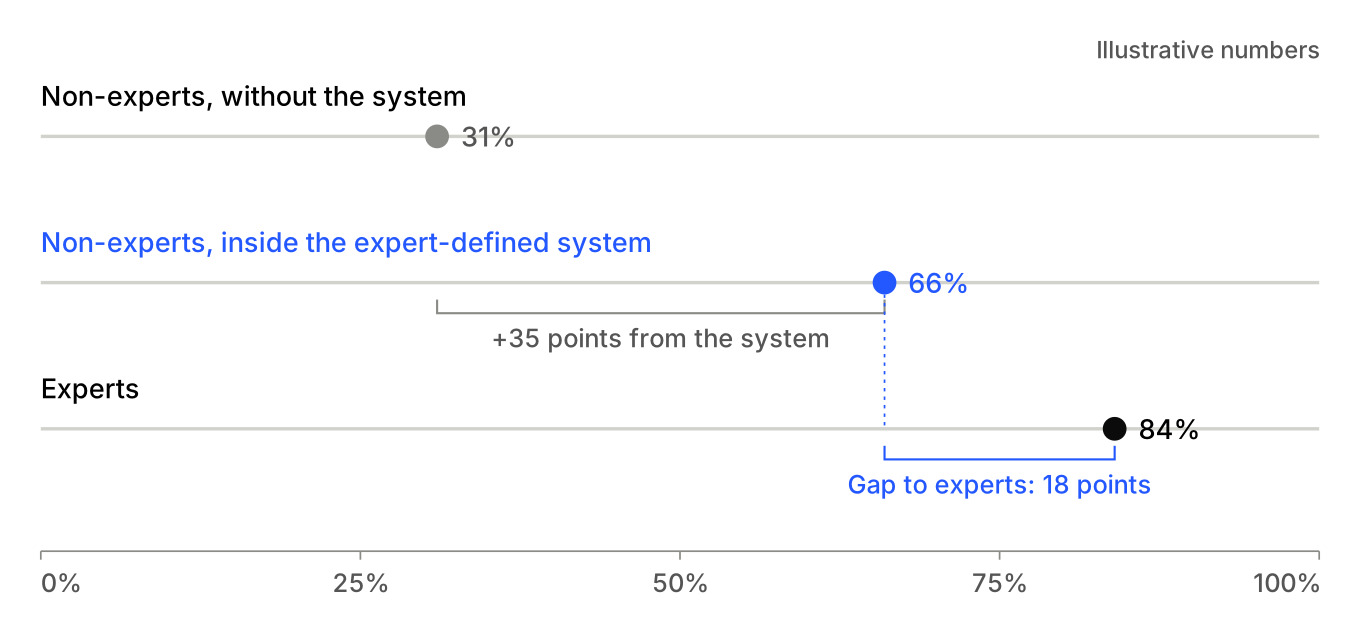
Dot plot of first-pass acceptance. Non-experts without the system: 31%. Non-experts inside the expert-defined system: 66%, 35 points higher. Experts: 84%, 18 points above the non-experts inside the system. — Read NFA against two comparisons: the same non-experts without the system, and experts. The lift says the system helps; the gap to experts is the number to watch. Illustrative numbers.

The experiment worth running

A clean test should compare novice and expert operators using general-purpose AI, then compare both groups using an expert-defined production system. Add no-AI baselines where practical. Randomise equivalent tasks, control for complexity, time budgets and prior familiarity, and use independent reviewers who cannot see which workflow produced each result.

The resulting comparisons answer different questions: Does AI reduce individual task time? Does it improve absolute quality? Does expert-designed governance raise the proportion of acceptable work? Does it reduce review effort and cost? Do advantages persist across multi-step workflows and changing contexts rather than only in a single prompt?

The strongest result would not be an impressive screenshot. It would be more accepted work, at lower total cost and with fewer material failures, consistently reproduced across task types. A weaker or negative result would be equally informative: perhaps expert-defined systems cost too much to configure, constrain creativity unnecessarily, or introduce new errors through automated review.

What this means for expertise

Expertise does not simply disappear. Some of it becomes easier to access. Some is embedded into tools and copied at scale. Some becomes more valuable because it specifies the objective, sets the boundary, chooses the tradeoffs and carries responsibility for what gets shipped. Goldfarb and Lindsay make a related argument about the complementarity of cheaper prediction and human judgment in decision-making. [4]

The better claim, therefore, is not that every expert wins or that novices are permanently behind. It is that people and organisations able to translate hard-won judgment into dependable systems may gain a different kind of advantage: quality, reliability and scale together.

That does not replace expertise. It scales it.

That is the problem we are working on with RepliKit. Expert-authored brand and production rules should be reusable. Review systems such as Kitana should make compliance and quality observable, while preserving escalation paths where the machine cannot safely decide. Those are product ambitions, not demonstrated customer outcomes until we measure them.

AI expands what people can generate. Expertise can help determine what is worth shipping. Systems decide whether that standard holds at scale.

What the mathematics does not prove

The mathematical framework is descriptive. Once a design space, feasible region and evaluation function are defined, optimisation within that region follows naturally. The equation does not establish that constraints are inexpensive to specify, that reviewers are correct, that experts always have better judgment, or that formalised systems outperform unconstrained generation.

Those are empirical hypotheses, and they can fail. They fail if the setup and maintenance costs exceed the savings. They fail if unstructured AI plus light review performs just as well. They fail if quality gates reject good work or approve dangerous work. They fail if an organisation cannot agree on which objectives matter.

But those hypotheses are measurable. We should measure productivity and quality in the same experiment, with the same standards, and follow the results wherever they lead.

References

Noy, S., & Zhang, W. (2023). “Experimental evidence on the productivity effects of generative artificial intelligence.” Science 381(6654), 187–192. Source
Brynjolfsson, E., Li, D., & Raymond, L. (2025). “Generative AI at Work.” Quarterly Journal of Economics 140(2), 889–942. Source
Dell’Acqua, F., et al. (2026). “Navigating the Jagged Technological Frontier.” Organization Science 37(2), 403–423. Source
Goldfarb, A., & Lindsay, J. R. (2022). “Prediction and Judgment: Why Artificial Intelligence Increases the Importance of Humans in War.” International Security 46(3), 7–50. Source
Lee, H.-Y., et al. (2020). “Neural Design Network: Graphic Layout Generation with Constraints.” ECCV. Source
Chen, C., Yan, X., Qi, X., & Cao, N. (2026). “IDEA: Automated Design Space Exploration for Visualization Design.” IEEE TVCG 32(7), 6566–6580. Source
Peng, Y.-H., Bigham, J. P., & Wu, J. (2025). “DesignPref: Capturing Personal Preferences in Visual Design Generation.” arXiv preprint. Source
Catalini, C., Hui, X., & Wu, J. (2026). “Some Simple Economics of AGI.” arXiv working paper. Source

Editorial note. This revision separates published empirical findings from mathematical formalisation and from product hypotheses. Example quality scores are fictional. The models and proposed metrics are analytical tools, not results of a completed RepliKit experiment.